
Graph for LLM (2)
Published:
Chinese version is in Zhihu 中文版
Graph for LLM (2)
This update is essentially a lightweight tutorial on using graph-based methods to study LLMs. The motivation came from being genuinely stunned by Anthropic’s March release, On Biology of a Large Language Model. Since my previous work all about graphs, I naturally wondered whether this attribution-graph idea could be extended and explored from a graph-centric perspective.
This blog-style tutorial walks through how we apply circuit-tracer methods to build graphs on top of LLMs and how these graphs can, in turn, influence LLM reasoning.
Recently, several papers have also started adopting circuit-tracer methods [1][2]. However, circuit tracing can feel extremely difficult when you first begin (at least it was for me — I spent a full month just figuring out the entire workflow from training to inference). So I organized the code and put together a minimal, beginner-friendly tutorial. https://github.com/DDigimon/GraphGhost
The core idea of this code tutorial is to make circuit tracing accessible even for people without large compute resources. For example, in the first module you can train a baby GPT model tailored to a specific task, and the whole pipeline runs on a single 3090 (about 20 GB of VRAM; even less if you reduce the number of layers or sequence length).
For the second part—graph construction—we also provide some of the graphs we generated ourselves, so you can combine them with the code to build the attribution graphs locally. We’ve run PageRank on these graphs for simple analyses, but of course there are countless graph algorithms and analysis methods. It feels like there’s a lot of room to try things and potentially discover something new.
The codebase is organized into two modules:
How to train your own synthetic-based transformer and interpret it using circuit tracers, and
How to apply circuit tracing directly on pretrained or finetuned LLMs, and what you can do with the graphs obtained from this analysis.
Synthetic data
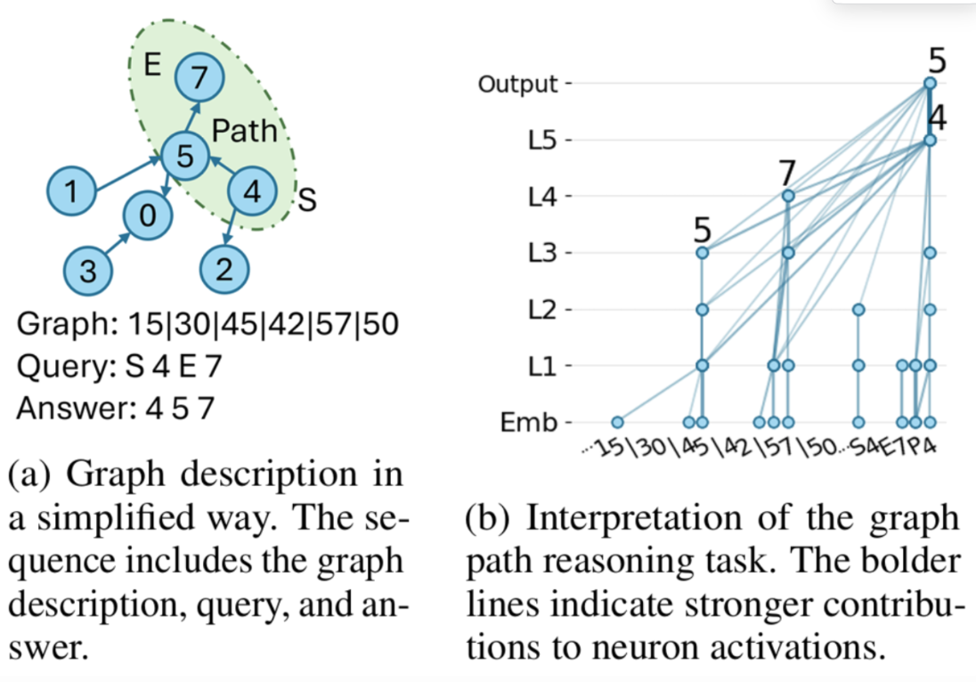
The code is located under simplified_graph_task. The main references are the tutorial and vis_example files. In this tutorial, we use a path-reasoning task on graphs as the running example.
The setup is as follows: suppose we already have a synthetic graph (as in figure a). Given the edge-list representation of the graph and a start–end pair for the path you want to predict, a Transformer should, in principle, be able to output the correct path. In figure b, we apply circuit tracing for interpretation and observe that the Transformer actually performs token merging internally to combine information across the sequence.
So this part of the code focuses on implementing these two components:
training the Transformer to perform path reasoning on the graph, and
using circuit tracer to analyze how the model merges and uses information internally.
First, we construct the dataset entirely from scratch. Ideally, the dataset should be sufficiently large and satisfy certain constraints. In our case, we start with a base graph containing 10 nodes and randomly sample subgraphs from it. During subgraph sampling, we randomly mask out some edges and nodes so that each sample becomes a different subgraph derived from the same large graph.
For the path-reasoning part, we only select paths of length greater than 2. In total, we sampled around 1,000,000 examples (though in reality you could probably use fewer it still works).
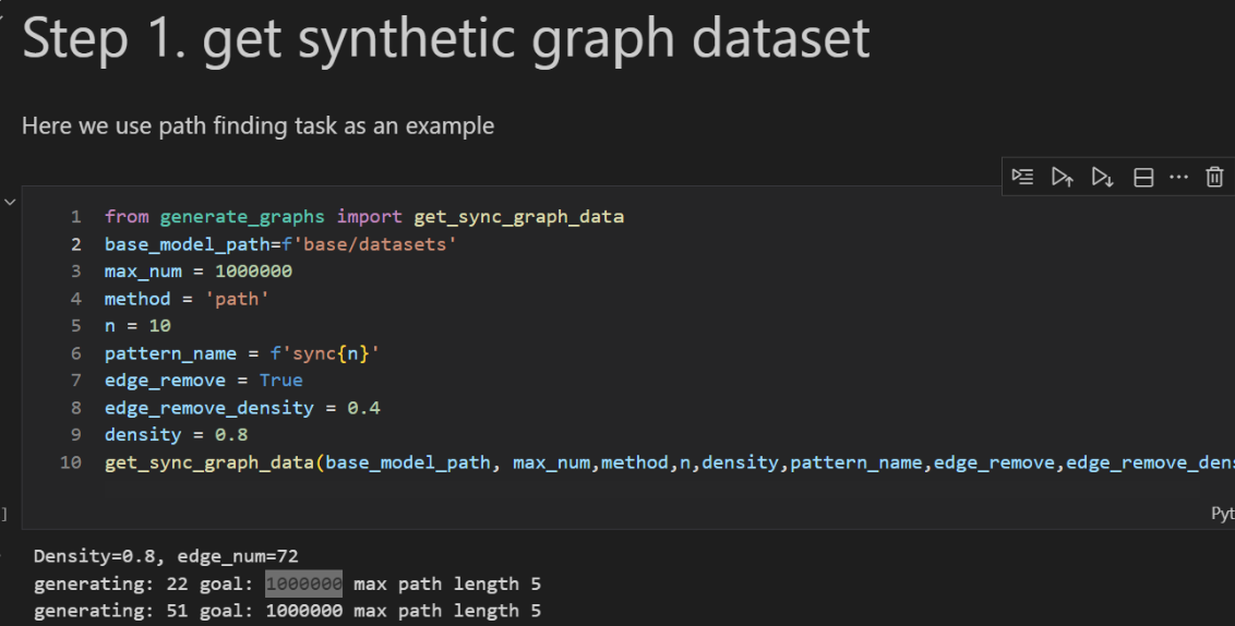
After that, we can start training. When training your own Transformer, you can refer to nanoGPT, which provides many useful small tips. In our case, the training framework is HookedTransformer. It is adapted from the original Transformer package to make the later circuit-tracer construction easier.
(As a small tip: HookedTransformer tends to be slower during training compared to a standard Transformer. So another option is to first train a normal Transformer and then port the weights into a HookedTransformer model afterward.)
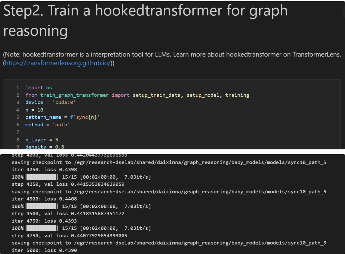
With this setup, the model converges in roughly 5k steps, and the evaluation accuracy can reach around 99%. One thing to note: the batch size must be large—if it’s too small, the model won’t train properly.
Once this basic Transformer is trained, you can start training the transcoders. Anthropic’s implementation uses a cross-layer transcoder, meaning all layer-level transcoders are stitched together into one large model and trained jointly.
However, in July a third-party implementation was released showing that you can also train one transcoder per layer and then assemble them at inference time. This codebase follows that approach: training a separate transcoder for each layer.
If you want to train the full cross-layer transcoder, you can modify the code accordingly. (I tried this once, but the computational cost was enormous, so I eventually abandoned it.)
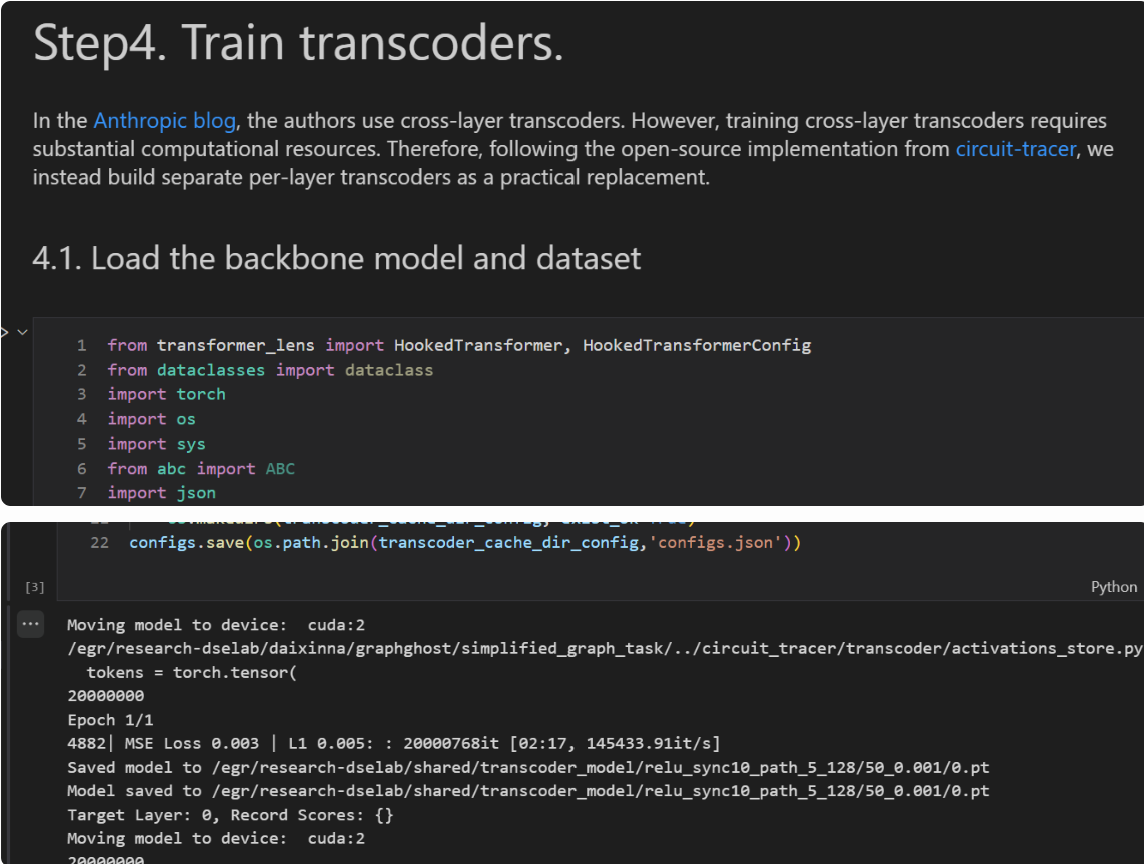
For transcoder training, the MSE loss for layer 0 usually reaches around 0.001, which is already good enough; the L1 loss can be pushed a bit lower as well. Ideally, we should have an evaluation script here, but the code is honestly too messy at the moment, so it remains on the TODO list. The core idea behind transcoder training is simple: you want the transcoder to learn from as many tokens as possible, so total_training_tokens should be made as large as you can. You’ll also need to tune dead_feature_window and l1_coefficient depending on the model size. If the MSE stops decreasing but L1 suddenly explodes, then you likely need to adjust the L1 coefficient. Another hyperparameter is d_transcoder. In practice, it doesn’t seem extremely sensitive—smaller values still train—but based on open-source implementations, a good rule of thumb is to set it to about 3× the model dimension, though this might depend on dataset size and other factors.
Once all of this is prepared, we can move on to visualization and analysis. The visualization code investigates the internal information flow when predicting the next token. For example, in the path-reasoning case shown, if the model predicts that the next token should be 0, how is that information internally propagated? This computational-flow graph corresponds to the implicit structure the model uses when generating the current prediction.
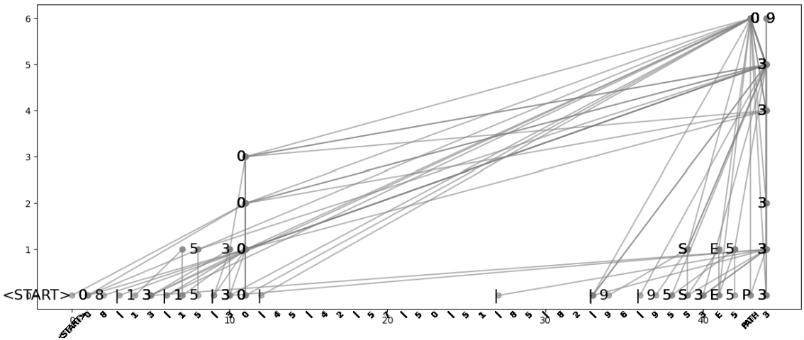
The idea is that the model discovers that there is an edge between 3 and 0, and it merges this information internally to influence the next-token prediction. (The figure shown here is a very rough visualization; the one in the introduction is manually tuned to look nicer. If needed, you can adjust the visualization parameters yourself.)
Two important parameters here are node_ratio and edge_ratio, which control the sparsity of nodes and edges in the implicit structure. Since the filtering process is based on ranking, these ratios determine how much of the attribution graph is kept. For details, you can refer to Anthropic’s blog.
LLM applications
Next is the LLM part. Methods like transcoders and SAEs have already been widely applied to interpret LLMs. But since my previous work are in the graph world, my first instinct was: can we interpret these behaviors as token walks on a graph?
At the simplest level, many recent works suggest that “thinking” in LLMs resembles a graph or a chain. So can circuit tracing help reveal a more intuitive, graph-like reasoning process inside LLMs?
On the other hand, if an LLM is effectively walking on an implicit graph, then in principle that graph should allow us to directly control the model’s behavior. And many graph algorithms could potentially be reused to enhance LLM reasoning.
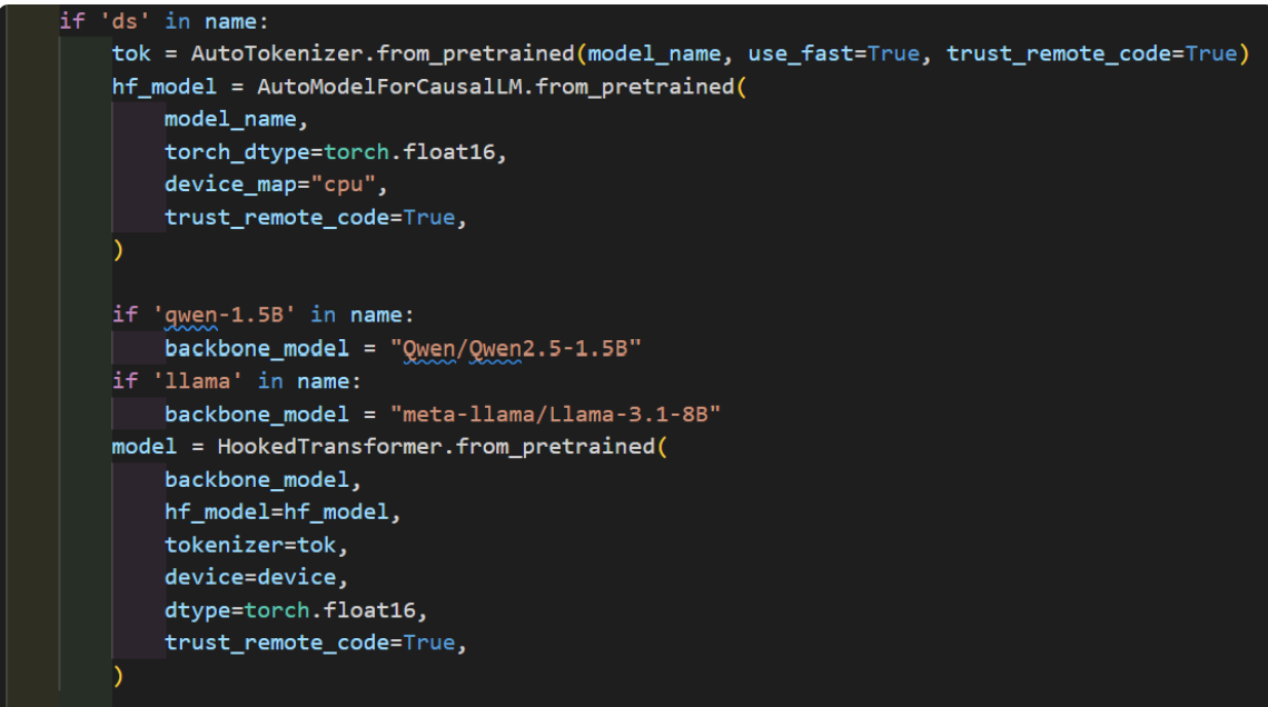
Since we don’t need to generate synthetic data here and the LLMs already exist, we can use them directly. How much interpretability we can extract simply depends on how many models are supported by the TransformerLens toolkit.
Finetuned models also work, because HookedTransformer is an extended Transformer implementation—so as long as the architecture matches, the weights can be loaded. For example, in our demo we successfully loaded a DeepSeek model.
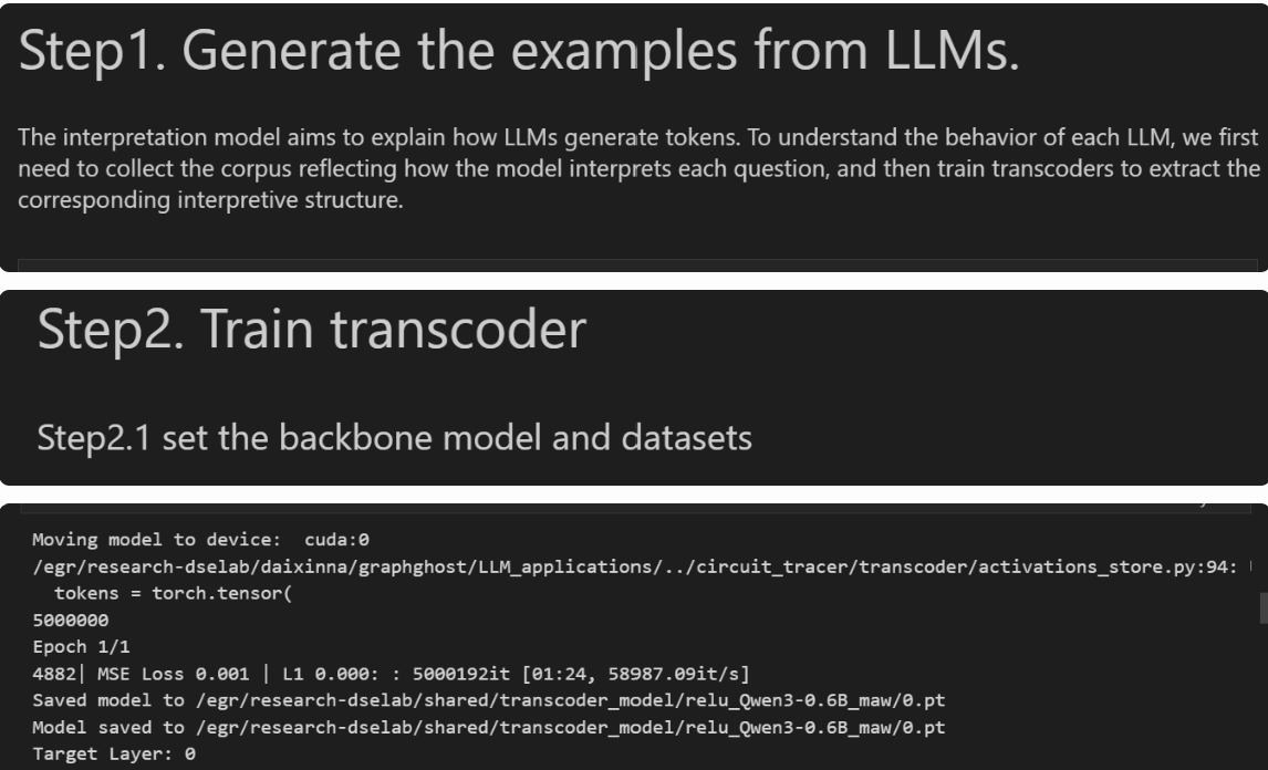
To match the model’s own output behavior, we first need to collect how the LLM actually answers questions. These responses must be gathered and used as the corpus for training the transcoders. After that, the second step is to train the transcoders—same process as before, just with different hyperparameters depending on the specific model and dataset.
At this stage, we no longer focus on visualization. Instead, we directly extract and package all the implicit structures produced by the model.
Because the attribution graph describes how the model predicts the next token, we need a way to trace back the entire reasoning process. For example, consider the math expression 1 + 2 + 3. The final answer is 6—but why 6?
Because the model internally reasons that 2 + 3 = 5, and then 1 + 5 = 6. Here, the token 5 is an intermediate reasoning step: it is not part of the original input (1, 2, 3), but it belongs to the chain of thought the model constructs. So when explaining the reasoning chain, we still need to trace why the model predicted 5. Tracing this will lead us back to the input tokens 2 and 3.
However, not every token in the chain-of-thought, nor every token in the original input, actually contributes to the final result. Therefore, we define a special subset called contribution tokens—the tokens that genuinely influence the implicit computation graph.
Once these contribution tokens are identified, we can collect the corresponding implicit structures based on them.
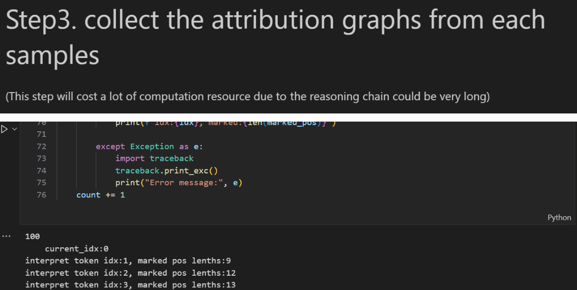
The logs here show messages like “Explaining token x” and indicate how many contribution tokens are still waiting to be processed. This step is actually quite resource-intensive. For that reason, we’ve already uploaded some decoded results to HuggingFace—you can download them and proceed directly to later analysis or perturbation experiments without running the full decoding pipeline yourself.
Now we reach the analysis stage. Here we mainly study two things:
Contribution tokens (as discussed earlier), and
Whether the LLM can build a coherent understanding of the entire dataset space.
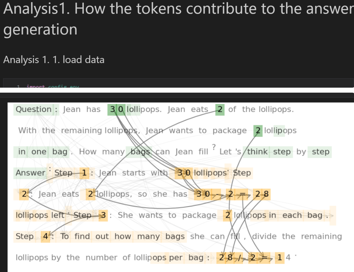
The first part is relatively straightforward: once we identify the contribution tokens, we simply connect them based on the recovered attribution structure. In our visualization, we use orange and green to distinguish tokens that come from the original sentence versus tokens that belong to the model’s chain-of-thought. (The edges themselves don’t have weights— they’re just drawn thicker to show the flow of information more clearly.)
This part corresponds to perturbing the input question. Long before modern LLMs, interpretability research used evaluation metrics called Fidelity and Sparsity. The idea was: if you remove part of the input data, does the model still stay faithful to its original prediction? This helps determine whether an interpretability method truly captures the input features that matter.
We can apply the same idea here: keep only the contribution tokens from the question and see whether the model’s output changes. For example:
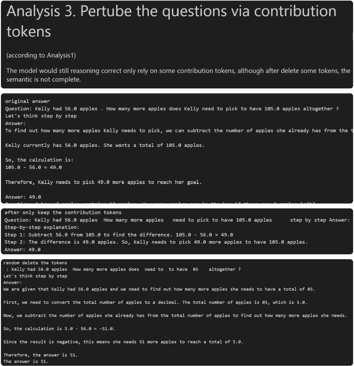
These three outputs correspond to:
the original answer,
the answer when only the contribution tokens are kept, and
the answer when we randomly mask tokens while keeping the same sparsity.
In the contribution-only version, the total number of tokens is much smaller. Even though the resulting sentence may not be very readable to humans, the model’s reasoning outcome remains consistent.
The second analysis aggregates multiple samples. From a dataset-level perspective, we want to see which tokens the LLM tends to collect at which layers. Here we used 100 samples to construct a “dataset-view graph” and ran a PageRank algorithm on it.
Since PageRank is designed to identify key nodes in a graph, we use it to find the most influential nodes in this implicit reasoning structure. This leads to the result shown.
Each explicit token in this graph is represented as a combination of the token itself plus its layer index. In a fully standard transcoder formulation, we would also include the feature dimension, but for simplicity we omit that here.
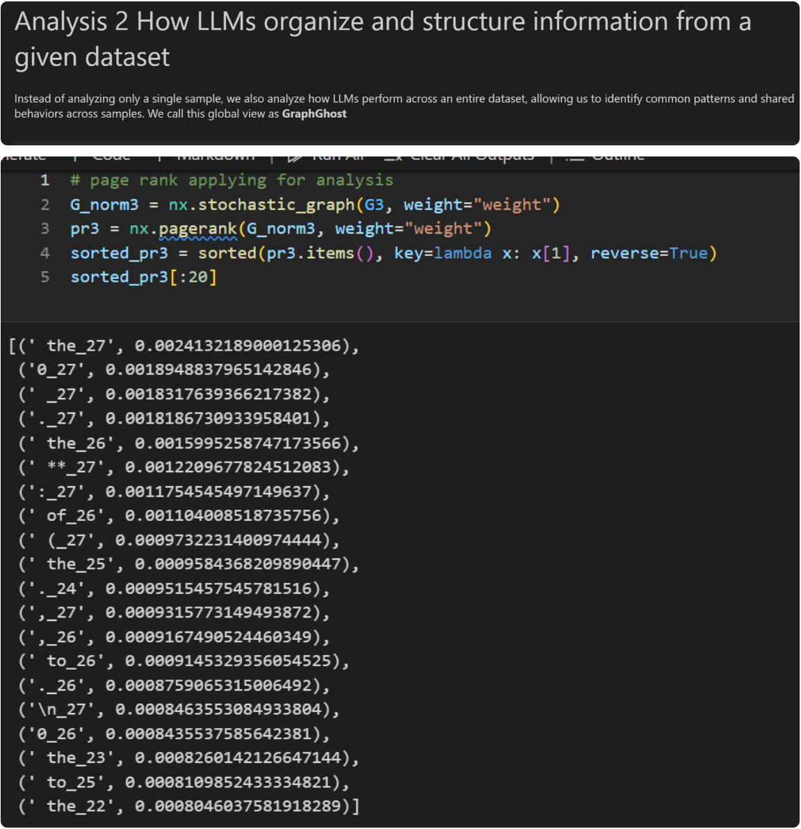
From this, we can observe that LLMs show clear preferences for certain nodes. For example, they tend to favorite high-layer nodes, which is a well-known phenomenon at this point. We also notice that the model strongly gravitates toward certain specific tokens, including seemingly meaningless ones like “the” or “to”.
With these analyses in hand, we can directly issue instructions to the LLM. For example: when the input token is “the”, block the neurons in layer 17.

Here’s a random example we tested: you can see that the LLM directly changes its reasoning logic after the intervention. It first provides a high-level overview, then details, and even switches from using the multiplication symbol to writing out “times”. This suggests that if we want to modify an LLM’s output style, sometimes a single neuron intervention is enough.
Alright, that’s everything included in the current version of the repo. More DLC may come later. There are still many things we haven’t done—for example, there are tons of interpretability methods, but we only tested the simplest combination: ReLU + transcoder. And the ReLU part really should evolve into JumpReLU or something more modern. For now, the goal was simply to get the basic tooling implemented.
The project is named GraphGhost partly because the entire idea is about making graphs serve LLMs, and partly because this “graph-building spirit” still seems to haunt everything in a surprisingly useful way.
We’ll later update with more “graph for LLM”–related paper repos and continue exploring whether looking at LLMs through a graph lens can uncover new ideas. If you’re interested, feel free to meet up and chat in San Diego!
### [1] Verifying Chain-of-Thought Reasoning via Its Computational Graph (https://arxiv.org/pdf/2510.09312) [2] Weight-sparse transformers have interpretable circuits(https://arxiv.org/pdf/2511.13653)
======